BioSens User’s Guide
UCSB’s BioSens:
A Toolkit for Sensitivity Analysis
(A Contribution to the Bio-SPICE Dashboard)
- Overview
- Installation Instructions
- BioSens Documentation
- Loading BioSens in Bio-SPICE Dashboard
- BioSens Tool
- Sensitivity Tool using XPP Simulator
- Sensitivity Tool using DASPK Simulator
- Plot Tool
- FIM Tool
- Options Tool
- Output Format
- Use Case
- Simple Circadian Rhythm Model
- Frog Egg Model
- Contact Information
1. Overview
BioSens provides a simulation and sensitivity analysis toolkit for Bio-SPICE through the BioMat Bridge. To simulate the dynamics of a biological system, BioSens uses one of two ODE-solvers – XPP or DASPK. XPP is a collection of differential equations solvers, developed by Bard Ermentrout at the University of Pittsburgh. DASPK is a differential algebraic equation solver with built-in sensitivity analysis developed by Shengtai Li and Linda Petzold at UC Santa Barbara. XPP will be used for models given in XPP format (.ode) and DASPK for SBML-2 models (.sbml or .xml).
Sensitivity analysis investigates the changes in the system outputs or behavior with respect to the parameter variations, which are quantified by the sensitivity coefficients S. Mathematically, the sensitivity coefficients are the first order derivatives of the outputs with respect to the system parameters:
![]() where yi is the i-th output and pj is the j-th parameter. When the model is described by an ordinary differential equation , the sensitivity matrix S can be derived from the model according to
where yi is the i-th output and pj is the j-th parameter. When the model is described by an ordinary differential equation , the sensitivity matrix S can be derived from the model according to
This sensitivity equation is solved directly in the implementation of the DASPK code. For XPP models, the toolkit implements centered difference approximation to compute the sensitivity coefficients:
The parameter perturbation magnitude Δp should be small enough to ensure small truncation error in the finite difference approximation, and large enough to reduce dependence on the simulation inaccuracies. We recommend using SBML models, as DASPK’s computation of the sensitivities is more accurate.
BioSens also includes Fisher Information Matrix (FIM)-based sensitivity analysis. Though the FIM was originally used to represent the amount of information contained in a given set of signals/measurements about the model parameters, it also can be interpreted as a consolidation of the system sensitivities. In this case, the FIM takes into account the underlying distributive nature of states or measurements due to the inherent stochasticity of cellular processes involving reactions with low copy number of substrates (McAdams, H. H. and A. Arkin, Trends Genet. 15:65-9, 1999) as well as noise in the measurements. The FIM-based sensitivity measures can give insights into the robustness and fragility trade off in biological regulatory structures based on the rank-ordering of the sensitivities (Stelling, J., E. D. Gilles and F. J. Doyle III, PNAS.101:13210-15, 2004). For ease of use, BioSens functionalities are accessible through a Matlab graphical user interface.
In addition, BioSens provides a measurement selection tool that selects the optimal measurement set for maximum parameter identifiability and accuracy. The purpose of this tool is to provide a feedback from a biological model to guide the next experiment for parameter refinement. The tool also uses the FIM, but here in the original interpretation as a measure of information. Given a limited set of measurements and their approximate accuracies, the tool can maximize two possible criteria for information (D- or A-optimality) such that the parameter estimation problem based on the measurements will give the most identifiable parameter set and the highest accuracy. Such tool allows an iterative procedure for model identification in which the knowledge from each iterate will be used to better design the next experiment for model refinement.
For more information about sensitivities and Fisher Information Matrix, the user can consult the following references:
- A. Varma, M. Morbidelli and H. Wu, Parametric Sensitivity in Chemical Systems, Cambridge University Press, Cambridge, U.K., 1999.
- L. Ljung, System Identification: Theory for the User, 2nd. Ed., PTR Prentice Hall, Upper Saddle River, N.J., 1999.
For more information about XPP and DASPK, consult:
- XPP: http://www.math.pitt.edu/~bard/XPP/XPP.html
- DASPK: http://www.engineering.ucsb.edu/~cse/software.html
2. Installation Instructions
a. Full Installation (Windows Only)
- Prerequisites:
- BioSens release file (BioSens.zip for Windows)
- Latest release of Bio-SPICE dashboard with BioMat Bridge
- Matlab (BioSens is tested to run in Matlab 6.5 R13 or Matlab 7.0 R14)
- XPP simulator (http://www.math.pitt.edu/~bard/XPP/XPP.html)
- Cygwin (http://www.cygwin.com)
- libSBML (http://www.sbml.org/libsbml.html)
This is used to parse the SBML input files.
Note: There are two versions of the libSBML – one that uses the Xerces XML parser, and one that uses Expat. We use the Xerces version.
DASPK is a collection of Fortran 77 routines that solve and perform sensitivity analysis on ordinary differential equations (ODE’s) and differential algebraic equations (DAE’s) s. It is subject to copyright restrictions, but is available for research purposes.
- Tapenade 2.1 (http://www-sop.inria.fr/tropics/tapenade.html) (optional)
Tapenade is an automatic differentiation package used to make DASPK simulations more efficient (by providing the Jacobian matrix of the system). It has been implemented as an on-line tool, but it is possible to download the .jar files and install it locally. If automatic differentiation is to be used, BioSens requires Tapenade to be installed locally. If Tapenade is not installed, then DASPK can approximate the Jacobian numerically.
- Install XPP:
- Go to http://www.math.pitt.edu/~bard/XPP/XPP.html.
- Decompress the distributed packages in the desired directory.
- Install Cygwin (version 1.5.14-1 or later)
- Download and run Setup.exe from http://www.cygwin.com
- In the “Select Packages” step, expand the list for Devel and select:
- gcc: C compiler
- gcc-g77: Fortran compiler
- make: the GNU version of the ‘make’ utility
Selection of these packages will automatically install other supporting packages.
- After finishing cygwin installation, add the cygwin path in the computer’s path environment variable. In Windows XP, this should be done as follow:
- Right click on “My Computer” and select Properties
- Go to the “Advanced” tab and proceed to “Environment Variables”
- In the System Variables table, highlight the Path variable, and press edit.
- At the very end of this variable, append the directory cygwin/bin, e.g., if cygwin is installed in “c:\cygwin”, then append “c:\cygwin\bin”. Remember to put the semicolon to concatenate the path.
Note: If you already have cygwin installed, it may be necessary to reinstall it to make sure the version is recent enough. There are problems calling Tapenade with older versions of cygwin.
- Install libSBML:
- Go to http://www.sbml.org/libsbml.html.
- Download and run the libSBML installer, using the typical installation method. Be sure the java bindings are installed.
Note: There are two versions of libSBML – one based on Xerces and the other based on Expat. We use the Xerces version. As of May 2005, the Windows installer for libSBML includes Xerces, making this installation the simplest.
- Install DASPK:
- Create the root DASPK directory (e.g. C:\DASPK).
- Go to http://www.engineering.ucsb.edu/~cse/software.html.
- Download daspk31.tgz by right-clicking on the link to DASPK 3.0. Select Save-As and save the file as daspk31.tgz in the root DASPK directory you just created.
- In cygwin’s BASH shell, the package can be expanded using the commands:
gunzip daspk31.tgz
tar -xf daspk31.tar
- There is no need to compile the code at this time. BioSens will do that for you.
- Install Tapenade (optional):
- Go to http://www-sop.inria.fr/tropics/tapenade.html for a brief introduction to the program. At the bottom of the page is information about installing Tapenade locally.
- Follow the link to their FTP server (http://www-sop.inria.fr/tropics/tapenade.html).
- Download tapenade2.1.tar.gz.
- Decompress tapenade2.1.tar.gz in the desired directory.
- Decompress BioSens release file, BioSens.zip, which will create a directory named “BioSens”. The directory should include
- BioSens.xml (wrapper for the BioMat Bridge)
- BioSensWithInput.xml (wrapper for the BioMatBridge)
- matlab folder containing the main BioSens implementations
- jars folder containing the supporting java code
- DASPK_Support folder containing DASPK-related BioSens code
- models folder containing example models such as circadian rhythm (tyson.ode) and frog egg (frogegg.sbml) use cases
- docs folder containing the documentation
b. Partial Installation (Windows or Unix)
It is possible to run BioSens with XPP-based tools only. In this case, one needs to have only Matlab, BioSens.zip, and xpp available to them. This option is designed for users who do not have Administrator privilege, those who have only small models, and/or those who are running in a Unix environment (Note: full installation should soon be available for Unix).
If the user has input files in SBML, then libSBML and java must be installed. This is a simple task for Windows, but is more complicated with Unix.
- Prerequisites:
- BioSens release file (BioSens.zip for Windows)
- Latest release of Bio-SPICE dashboard with BioMat Bridge
- Matlab (BioSens is tested to run in Matlab 6.5 R13 or Matlab 7.0 R14)
- XPP simulator (http://www.math.pitt.edu/~bard/XPP/XPP.html)
- Install XPP:
- Go to http://www.math.pitt.edu/~bard/XPP/XPP.html.
- Decompress the distributed packages in the desired directory.
- Install libSBML (for SBML model files):
- Go to http://www.sbml.org/libsbml.html.
- Download and run the libSBML installer, using the typical installation method. Be sure the java bindings are installed.
Note: There are two versions of libSBML – one based on Xerces and the other based on Expat. We use the Xerces version. As of May 2005, the Windows installer for libSBML includes Xerces, making this installation the simplest.
- Decompress BioSens release file, BioSens.zip, which will create a directory named “BioSens”. The directory should include
- BioSens.xml (wrapper for the BioMat Bridge)
- BioSensWithInput.xml (wrapper for the BioMatBridge)
- matlab folder containing the main BioSens implementations
- jars folder containing the supporting java code
- DASPK_Support folder containing DASPK-related BioSens code
- models folder containing example models such as circadian rhythm (tyson.ode) and frog egg (frogegg.sbml) use cases
- docs folder containing the documentation
3. BioSens Documentation
a. Loading BioSens in Bio-SPICE Dashboard
In the Bio-SPICE Dashboard (consult the Bio-SPICE release manual for starting the dashboard):
- Open the Workflow Editor (in dashboard, go to Bio-SPICE -> Open Workflow Editor).
- Drag the BioMat Bridge icon onto the workflow.
- Right click on the BioMat Bridge to open the BioMat Bridge Configuration window (select Edit -> Analyzer Configuration).
- Load the file BioSens.xml in the BioSens folder (by clicking Load in the Configuration window). BioSens.xml provides a standalone toolkit which does not produce output to the dashboard. It does, however, write to several output files in the form of Matlab and ASCII text files. Please refer to the Output format section for further details.

- Go to the Search Paths tab in the BioMat Bridge Configuration window
- Start the workflow. If this is the first time BioSens is loaded, the Preferences Tool will be opened and the user will be prompted for the location of five folder/files:
- Root installation directory of BioSens
- libSBMLj.jar – the libSBML Java bindings
- Root installation directory of DASPK
- XPP executable (this is typically called “xppaut.exe”)
- Root installation directory of Tapenade
Note: For the partial (XPP-only) installation, simply leave the DASPK and Tapenade paths blank.
This path information is physically stored in the preferences file (BioSensToolPrefs.txt) under Matlab’s default preference folder (specified by Matlab’s prefdir function).
The Preferences Tool also provides the option of having status messages written to Matlab’s Command Window (in addition to the status bar at the bottom of each tool). This is available because Matlab’s Command Window often displays messages before the tool’s user interface displays them.
b. BioSens Tool
The main window of BioSens allows the user to:
- Load a model (in SBML Level 2, XPP *.ode, or BioSens *.bsn)
- Calculate the sensitivity coefficients of the model using finite difference approximations. The user can compute the system sensitivity with respect to the model parameters as well as the initial conditions. This button will spawn one of two different windows, depending upon the input format.
- Compute the Fisher Information Matrix and obtain FIM-based sensitivity measures.
- Select the optimal measurement set for parameter estimation.
- Edit the Preferences of the BioSens toolkit (under the Edit menu).
Details:
- Menus
- File
- Open: Load a model (*.ode; *.sbml; *.xml; *.bsn)
- Close: Close BioSens (all BioSens related windows).
- Edit
- Preferences: Brings up the Preferences dialog box.
- About
- Provides version and contact information for BioSens.
- File
- Loading a Model in BioSensBioSens accepts input files in three formats:
- SBML Level 2 Files with the following restrictions:
- Each reaction must have a kinetic law
- If units are present, they must be consistent. (Units are ignored by BioSens.)
- SBML Level 2 Files with the following restrictions:
It is worth noting that there is no need for the writer of an SBML file to determine which species are independent (require an ODE) and which species are dependent (can be computed algebraically from concentrations of other species). BioSens will automatically detect dependent species. The code for this is based on Herbert Sauro’s Structural Analysis Part II: Conservation Relations and modeled after the implementation by Marc Vass (as part of the JigCell project).
When BioSens reads in an SBML file, it invokes a parser to generate both *.ode and internal *.bsn versions of the model. It then automatically load the *.bsn version of the file, which user can (and should) use the in subsequent runs.
References
- http://www.cds.caltech.edu/~hsauro/Algorithms/struct1.pdf
- http://jigcell.biol.vt.edu/
- BioSens *.bsn internal format.
*.bsn is a text format designed to minimize the time required to load a model into BioSens. This means the easiest and most efficient way to use BioSens is to load in the SBML version of a file the first time you analyze it in Biosens. Thereafter, load the .bsn version of the model.
- XPP *.ode files with the following restrictions:
- Differential equations should start with the format, e.g., d<state>/dt = …
- Parameters should be specified separately, one parameter each line, e.g., param <param name>=<param value>
- Initial conditions should also be written separately, one state per line, e.g., init <state>=<initial condition>(Note: The *.ode files created by JigCell conform to these restrictions.)
BioSens will create a working directory which will store the simulation data and the analysis results. If the selected directory exists, BioSens will load up saved simulations and results from the past run. The user can choose to clear up the working directory for a new run.
- Computing the sensitivitiesDepending on the format of the input, BioSens will bring up the window appropriate for its format. SBML and BioSens models are simulated using DASPK, while those in the XPP format are simulated with XPP. The next two sections cover the functionalities of the different solvers.
- Computing the FIMAfter the sensitivity matrix has been computed, the user can access the FIM Tool for computation of the Fisher Information Matrix and FIM-based sensitivity analysis.
- Measurement selection tool
Using the sensitivity matrix, this tool allows selection of the optimal measurement set to maximize parameter accuracy and identifiability.
- Closing the toolClosing BioSens main window (via the “Close” button or the “Close” menu option) will also close all BioSens related windows.
c. Sensitivity Tool using XPP Simulator
- Parameters
The controls in this frame allow the user to adjust the nominal values and perturbation magnitudes for each parameter in the finite difference approximation.- List Box: The list box contains the list of the model parameters with their names, nominal values, and perturbation magnitudes. Selecting the parameter in the list box allows the user to access the nominal value and the perturbation magnitude.
- Nominal Value: Set the nominal value for the selected parameter. The value must be numeric.
- Perturbation: Set the parameter perturbation magnitude for the selected parameter. The value must be numeric.
NOTE: The user can exclude a parameter from the sensitivity analysis by simply setting the perturbation value to 0.0. - Perturbation Unit: Select the unit for the perturbation magnitude.
- %: The parameter will be perturbed by a percentage of the nominal value.
WARNING: If the nominal value is 0.0, then perturbations should not be given in units of %. - Nom. Val. Unit: The perturbation value has the same units as the nominal value.
- %: The parameter will be perturbed by a percentage of the nominal value.
- Initial Conditions
The controls in this frame allow the user to adjust the nominal values and perturbation magnitudes for the initial condition of each state, which have the same functionality as in the Parameters control frame (see above). - XPP Simulation Parameters
This table shows the parameters for the XPP simulations (consult XPP manual for further details). All values (except the method) must be numeric.- Total: Total simulation time.
- Tolerance: Error tolerance for several of the integrators.
- Abs. Tolerance: Absolute tolerance for several of the integrators.
- Max Storage: Limits the total number of steps that will be stored in memory. The max storage should be at least (Total/dt)+1.
- dt: Time step of simulation.
- njmp: The integration step interval to written in the output file.
- t0: Starting time.
- Method: Method of integration.
- Bound: Upper bound for the absolute values of the states.
- Max Delay: Maximum time delay allowed. It is important to make this value large enough for any delay statements in the model. XPP uses the value of Max Delay to determine the extra storage requirements for the simulation. However, if it is too large, then XPP may use too much memory.
- Gear Min: Minimum allowable timestep for the Gear integrator (applicable only when the Method is set to “gear”).
- Gear Max: Maximum allowable timestep for the Gear integrator (applicable only when the Method is set to “gear”).
- Using the Options to Adjust Values:
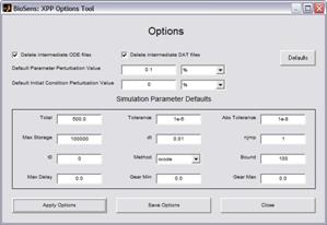
The Options dialog box (accessible through Edit menu) allows the user to change the default values for several BioSens parameters, as well the option to keep or delete temporary files. These settings can be changed on a “per session” basis, or, more permanently, by saving them to a file.
Details:
- Defaults: Restore the Options to the factory default settings.
- Apply Options: Upload the settings to the current BioSens window. These values will be used as default until the BioSens window is closed.
- Save Options: Upload the settings in the current BioSens window and save the settings for future BioSens sessions.
Note: The Options file (BioSensToolOptions.txt) is located in the folder returned by the Matlab function “prefdir”. - Close: Close the Options tool.
- Delete intermediate ODE files Checkbox: If checked, all temporary model *.ode files used in finite difference approximation will be deleted.
- Delete intermediate DAT files Checkbox: If checked, all temporary XPP simulation output *.dat files will be deleted.
- Computing Sensitivity:
Once the perturbation magnitudes and simulation parameters have been set, click the “Compute Sensitivity” button to run the simulations and compute the sensitivity coefficients. Computation can be stopped by clicking the “Cancel” button.
- Plotting Sensitivity:
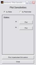
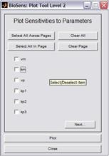
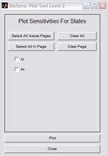
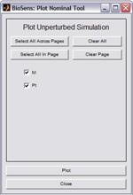
Once the sensitivity matrix has been computed, the user can access the Plot Tool via the “Plot Sensitivity” button. The Plot Tool can produce:
- For each state, a plot of the sensitivities with respect to the parameters and/or initial conditions.
- For each parameter/initial condition, a plot of the sensitivities of different states.
- A plot of the system dynamics with the nominal parameters and initial conditions.
d. Sensitivity Tool using DASPK
- Parameters
The controls in this frame allow the user to adjust the nominal values for each parameter in the model and select the parameters whose sensitivities should be computed. - Initial Conditions
The controls in this frame allow the user to adjust the nominal values for each initial condition of the states in the model and select the initial condition whose sensitivities should be computed. - DASPK Simulation Parameters
This table shows the parameters for DASPK simulations:- Total: Total simulation time.
- dt: Time step of simulation.
- Tolerance: Relative tolerance of simulation.
- Abs Tolerance: Absolute tolerance of simulation.
- Automatic differentiation: Options to use Tapenade automatic differentiation of the system’s Jacobian in the simulation. This is generally more accurate than the default finite difference method.
- Using the Options to adjust values
The options dialog under edit menu allows adjustments of the default values of simulation parameters. The functionality is similar to the XPP options.
e. Plot Tool
The Plot Tool provides the ability to visualize the system dynamics and the sensitivities. This tool can be accessed from both the main BioSens and the XPP/DASPK simulation windows. It is possible to view:
- For each state, a plot of the sensitivities with respect to the parameters and/or initial conditions
f. Fisher Information Matrix (FIM) Tool
The FIM Tool provides the interface to compute the Fisher Information Matrix from the sensitivity matrix and user-provided standard deviations. The standard deviations represent the amount of noise in the measurements (in this case, the states). Under the Gaussian assumption, the FIM is computed according to:
FIM = STV-1S
where S is the sensitivity matrix and V is the covariance matrix:
such that n is the number states and NT is the total number of time steps. The FIM tool uses the Relative Error and Absolute Error to compute the standard deviation for the i-th state according to:
si,j = relative_errori × yi,j + absolute_errori
where yi,j is the nominal value of state i at time step j.
The FIM Tool is shown in the following figure. The user can edit the relative error for all states on the current page by setting the “Default Relative Error” field and clicking the “Apply to Page” button. To edit all the relative error for all states in the model, press the “Apply to All” button. Likewise, the user can edit the absolute error for all states on the current page, or all states in the model using the “Default Absolute Error” field and its related buttons.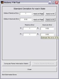
If the resulting FIM has moderate size, then it is displayed in a dialog box such as shown here:
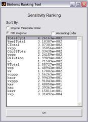
Clicking the button “Display Sensitivity Measure” will bring up the sensitivity rankings window. The FIM diagonal rankings are computed from the diagonal entries of the normalized FIM:![]()
where pi is the nominal parameters and m is the number of parameters.
The sensitivity measures can be sorted by the order of appearance in the BioSens main window, or by the FIM sensitivity measures by checking the appropriate choice.
g. Measurement Selection Tool
The purpose of this tool is to select the states in the model which represent the optimal (noisy) measurement set for parameter estimation. BioSens provides two choices of optimality criteria, practical identifiability and D-optimality. In practical identifiability, the optimal set is selected to give the best parameter accuracy as measured by the standard deviations. According to the Cramer-Rao theorem, the (inverse of) Fisher Information Matrix gives the lower bound for the variances in the parameter estimates from which the standard deviations can be computed. On the other hand, D-optimality criterion uses the determinant of the FIM as a measure of the information content in the states. Maximizing this criterion corresponds to maximizing the volume of information and thus the accuracy of the parameter estimates. In both cases, the number of identifiable parameters is maximized preceding to the optimization of the criteria.
The selection process is divided in steps.
- First step: the user provides estimates of the measurement error/noise needed to compute the Fisher information matrix
- Second step: Remove a priori unidentifiable parameters as they cause the FIM to become singular. These unidentifiable parameters correspond to the eigenvalues of FIM which are smaller than the identifiable tolerance.
- Third step: Further select the focus group among all identifiable parameters for which the optimal measurement should be selected. For example, if some of the parameter values have been accurately identified by independent measurements, then this set of parameters can be taken out of the focus group.
- Fourth step: For a given total number of measurements, BioSens will determine the states that will optimize the chosen criterion (practical identifiability vs. D-optimality) for the focus group of parameters.

Note that the parameters that will appear in the first step depend on the selection of parameters to which the sensitivities were computed and available, i.e., the parameters in the sensitivity computation step by either XPP or DASPK.
h. Output Format NOT DONE
Output Files:
The workspace directory will contain the following files:
- S#.mat: Contains the sensitivity matrix (in Matlab’s format) for the #-th state according to the ordering of the initial conditions in the BioSens main window. When XPP is used, S#.mat contains the sensitivity matrix as described below. When DASPK is used, S#.mat contain the transpose of the sensitivity matrix.
The columns of the sensitivity matrix consist of the sensitivity coefficients with respect to the model parameters and initial conditions in the order of the appearance in the BioSens window. The rows represent the time axis, which can be found in the file t.mat below. For example, the sensitivity matrix for i-th state of a model with perturbed parameters and perturbed initial conditions will have the following block structure: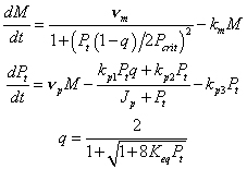
To load the information into Matlab, we use the code:
S = load(fullfile(subdirName,[‘S’,num2str(stateNum),’.mat’]));
if isfield(S,’S’)
% Collected with Xpp code
S = S.S;
else
% Collected with DASPK code
S = S.ST’;
end;
- t.mat: The time step vector in Matlab’s format.
The values are stored in different variables, and with slightly different formats, depending upon which simulator was used.
To load the information into Matlab, we use the code:
t = load(fullfile(subdirName,’t.mat’));
if isfield(t,’t’)
% Collected with Xpp code
t = t.t;
else
% Collected with DASPK code
t = t.ST’;
end;
- nominal.mat: The values of the system dynamics (output of simulation that uses unperturbed, or nominal parameters).
The values are stored in different variables, and with slightly different formats, depending upon which simulator was used.
To load the information into Matlab, we use the code:
nominal = load(fullfile(subdirName,’nominal.mat’));
if isfield(nominal,’nominal’)
% Collected with Xpp code
nominal = nominal.nominal;
else
% Collected with DASPK code
nominal = nominal.ST’;
end;
- fim.mat: The FIM in Matlab’s format.
- rankings.txt: The FIM based sensitivity rankings.
- nominal.ode and nominal.dat: The model with nominal parameters and the corresponding XPP simulation output, respectively.
- Optional *.ode and *.dat files of the model with perturbed parameters and/or initial conditions. For example, the “tyson” subdirectory may contain:
- tyson_dparam1.ode: ode file for 1st parameter with nominal value – perturbation value.
- tyson_dparam1_dat.dat: XPP output file
- tyson_uparam1.ode: Ode file for 1st parameter with nominal value + perturbation value.
- tyson_uparam1_data.dat: XPP output file
- xpprun.txt: The text output from the XPP simulations which may contain warnings or error messages from the simulations.
4. Use Case
a. Simple Circadian Rhythm Model (XPP Format)
The first example is a circadian rhythm model (J. J. Tyson, C. I. Hong, C. D. Thron, and B. Novak, Biophys. J., 77:2411-2417, 1999.). The model consists of 2 states with 9 parameters:
- Load BioSens in Bio-SPICE dashboard.
- Open tyson.ode file under the models folder included with the BioSens release. (If this is the first time of loading BioSens, the user will need to set the preferences as described above.) Use the default workspace directory. Then click on “Compute Sensitivities” button to access the XPP simulation window.
- In the XPP simulation window, go to Edit -> Options and change the following:
Click “Apply Options” and close the Options menu to put the changes into effect. The XPP window should look as in the following figure.
- Start the calculations by clicking the “Compute Sensitivity” button. This should take a couple of minutes to run depending upon the speed of your computer. The simulation status is displayed at the bottom of the main window.
- Once the simulations are done, the buttons “Plot Sensitivity” will become activated. Click on “Plot Sensitivity” to invoke the Plot Tool. Plotting the sensitivities by the state M with respect to the parameters vm and km gives

(Note: The sensitivities grow linearly with time as expected because the system evolves around a limit cycle. The system oscillates with a period of approximately 25 hours.)
- Close the XPP simulation window to go back to the main BioSens menu. Clicking on the “Compute Fisher Information Matrix” will bring up the Fisher Information Matrix (FIM) tool. Assuming that the measurements have relative error to 10% and absolute error of 0.02, we can proceed to compute the FIM. A window displaying the FIM will pop up. In addition, clicking “Display Sensitivity Measures” will give a sensitivity ranking based on FIM diagonal values (the square-root of the normalized FIM diagonals).

(Note: Sensitivity analysis here suggests that the system is most sensitive to the parameters km and kp3, related to the mRNA degradation and protein phosphorylation, and least sensitive to the parameter Keq, the dimerization equilibrium constant.)
b. Frog Egg Model (SBML format)
The second example uses the frog egg model provided by JigCell (http://jigcell.biol.vt.edu). Refer to the JigCell manual for details of this model.
- Load BioSens in Bio-SPICE.
- Open frogegg.sbml from the BioSens models folder. Use the default workspace directory. Proceed to click on the “compute sensitivities” button.
- In the DASPK simulation window, adjust the DASPK parameters to:
- Total: 100 (comment: total simulation time)
- dt: 0.5 (comment: time step size of the simulation output)
- Tolerance: 1e-6
- Abs. Tolerance: 1e-8
- Check on the automatic differentiation (make sure Tapenade is installed)
Click on the “select across pages” in the parameter section to automatically include all the parameters in the sensitivity computation. The BioSens main window should look as follows:
- Proceed to compute the sensitivity and plot the results (see Plot Tool). Here are samples of the results:
(Note: The figure on the left shows the plot of sensitivities of the state Ca to all parameters, while that on the right shows the sensitivities to the dilution parameters on all the states.)
- Invoke the FIM tool and set the relative error to 5% and absolute error to 0.01 for all states using the “Apply to All” button. The sensitivity ranking (by clicking the “Display Sensitivity Measure” button) suggests that the system is most sensitive to the parameter “TotalCycl” (see JigCell documentation for further details of the parameters involved).
- Next, proceed to the measurement selection tool. In the first step, assume that all states can be measured up to 10% accuracy and 0.1 absolute magnitude error. Using identifiability tolerance of 0.001, the tool will identify four unidentifiable parameters, leaving 14 parameters in step 3. After inclusion of all parameters in step 3, proceed to use the practical identifiability for optimization in the fourth step with a constraint of only 2 total measurements. The result shows that it is optimal to use the states Ma and Ca. (Exercise: repeat the whole procedure, but now with only the dilution as the focus parameter in step 3. The optimal measurement set for both practical identifiability and D-optimality is L and Ma. )

5. Contact Information
Prof. Francis J. Doyle III
Department of Chemical Engineering
University of California, Santa Barbara
Santa Barbara, CA 93106
Office: (805) 893-8133
Fax: (805) 893-4731
Email: frank.doyle@icb.ucsb.edu


